Lifetime Aggregations
Introduction
A lifetime aggregation is feature providing an aggregate calculation (e.g. sum, mean, min) over the full history of data for a given entity (e.g. total customer spend since acquisition).
Because lifetime aggregations process a lot of data, they can be difficult to implement efficiently. The biggest factor for determining how to implement a lifetime aggregation is how often data is inserted/updated for a given entity and how often each calculation needs to be refreshed. The recommended options for implementing batch and streaming lifetime aggregations are summarized in the table below.
| Type of lifetime aggregation | Recommended options for implementation |
|---|---|
| Batch | A Batch Feature View that uses a time-window lifetime aggregation or a custom lifetime aggregation. |
| Stream | A two-component solution: 1. A Stream Feature View using a time-window lifetime aggregation with a short time window to capture fresher signals. 2. A Batch Feature View using a custom lifetime aggregation that has a longer time window than the Stream Feature View to capture older signals. |
Approaches to creating lifetime aggregations
There are two main approaches to creating lifetime aggregations, which are discussed in the sections that follow.
Time-window lifetime aggregations
Time-window lifetime aggregations are built-in implementations of common
aggregations using time windows (such as count and sum). Time-window
aggregations can be used in
Batch Feature Views
and
Stream Feature Views.
- ✅ Simple implementation leveraging Tecton's managed time-window aggregations; lower learning curve
- ✅ Able to proxy lifetime aggregations when the lifetime horizon is short and data does not frequently change
- ❌ Inefficient at longer lifetime horizons and leads to high costs when underlying data changes frequently
- ❌ Limited to aggregate functions supported by Tecton's time-window aggregations
Implementing a time-window lifetime aggregation
Compared to the definition of a Feature View using a non-lifetime time-window aggregation, a Feature View using time-window lifetime aggregation is different in the following ways:
-
The
time_windowis set to early date that is on or around thefeature_start_time. -
batch_schedule(if set) andaggregation_intervalshould not be set to low values. (These parameters may be set to low values in a non-lifetime time-window aggregation Feature View). When these parameters are set to low values, the aggregation will run more frequently.
If you want to run a lifetime aggregation at a high frequency, using a custom lifetime aggregation is recommended instead.
Following is an example of a time-window lifetime aggregation.
@batch_feature_view(
    sources=[transactions_batch],
    entities=[user],
    mode="spark_sql",
    feature_start_time=datetime(2012, 9, 1),
    batch_schedule=timedelta(days=14),
    aggregation_interval=timedelta(days=14),
    aggregations=[
        Aggregation(
            column="amount",
            function="mean",
            time_window=timedelta(weeks=52 * 10),
            name="lifetime_",
        ),
    ],
    ttl=timedelta(days=35000),
    description="Lifetime user transaction amount (batch calculated)",
)
def tecton_managed_lifetime_count(transactions):
    return f"""
	    SELECT
	        user_id,
			1 as count_transaction,
			timestamp,
	    FROM {transactions}
	    """
Custom lifetime aggregations
If you want to run a lifetime aggregation at a high frequency, using a custom aggregation is recommended instead of using a time-window aggregation.
The implementation discussed below is supported on Spark (EMR or Databricks). Contact Tecton support if you are re interested in using custom lifetime aggregations on Snowflake.
Custom lifetime aggregations support all aggregations that are available on Spark. However, these aggregations do not leverage Tecton’s pre-computed tiles that are available in time-window aggregations and thus must be optimized using efficient Spark logic or with intermediate staging tables.
- ✅ Minimizes the amount of writes to the feature store, reducing costs (especially with data that changes frequently).
- ✅ Able to efficiently process data over any time horizon and process data
prior to the
feature_start_time - ✅ Flexible; able to process any aggregation supported by the underlying
transformation mode (
spark_sql,pyspark,snowflake_sql) - ❌ Complex implementation with high learning curve
Implementing a custom lifetime aggregation
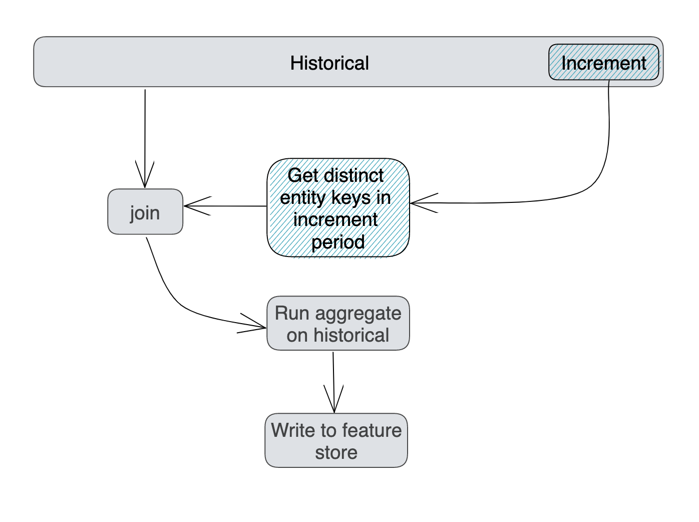
For efficiency, Tecton recommends designing the transformation logic to minimize the amount of data written to the feature store with the following pattern:
- Identify only the entities (such as user ids) that have been updated during the increment period.
- Read, from the underlying data source, the historical data for this subset of entities and perform the aggregation. The historical data includes the incremental data.
- Write the resulting aggregated values to the feature store.
This process is illustrated in the following diagram.
To ensure that the Feature View contains a lifetime aggregation for every entity (e.g. user id), during the first materialization job, the full historical data is processed for each entity. This is not shown in the diagram.

Example code implementation:
from tecton import batch_feature_view, materialization_context, FilteredSource
from fraud.entities import user
from fraud.data_sources.transactions import transactions_batch
from datetime import datetime, timedelta


@batch_feature_view(
    sources=[
        # Filters `transactions_batch` to the materialization period, i.e. [start_time, end_time).
        FilteredSource(transactions_batch),
        # Filters `transactions_batch` up to the end of the materialization period, i.e. [0, end_time).
        FilteredSource(transactions_batch, start_time_offset=timedelta.min),
    ],
    entities=[user],
    mode="pyspark",
    online=False,
    offline=True,
    timestamp_field="timestamp",
    feature_start_time=datetime(2022, 9, 1),
    batch_schedule=timedelta(days=1),
    incremental_backfills=True,
    # Use a very long TTL. The query is structure to only produce new feature values if the user has new data. Feature values are valid until they're overwritten.
    ttl=timedelta(days=3650),
    description="Last user transaction amount (batch calculated)",
)
def custom_agg_sample(source_deltas, source_historical, context=materialization_context()):
    """
    where T = feature_start_time (earliest time we support time travel with)

    distinct CTE: Identify distinct id's whose data has changed
                        backfill: pulls distinct user_id's who have had data change within the backfill increment
                        incremental: pulls distinct user_id's who have had data change in the past increment

    aggregation - recalculate lifetime aggregate for those id's who have changed
    """
    from pyspark.sql.functions import count, countDistinct, sum, lit
    from datetime import datetime

    # Manually copy the feature_start_time defined above
    feature_start_time = datetime(2022, 9, 1)

    # if first period: pull distinct id's in source data prior to feature_start_time
    # Else pull distinct list from materialization window defined by the FilteredSource
    is_first_period = feature_start_time == context.end_time

    if is_first_period:
        distinct_ids = source_historical.select("user_id").distinct()
    else:
        distinct_ids = source_deltas.select("user_id").distinct().limit(1)

    # pull the historical data prior to the window end
    historical_of_distinct_ids = distinct_ids.join(source_historical, "user_id")

    # Aggregate historical data at the time of the window end for each user
    aggregates = historical_of_distinct_ids.groupBy("user_id").agg(
        sum("amt").alias("lifetime_amt"),
        countDistinct("category").alias("lifetime_catg_distinct_count"),
        count("amt").alias("lifetime_transaction_count"),
    )
    # Add the window end time as the timestamp
    return aggregates.withColumn("timestamp", lit(context.end_time - timedelta(microseconds=1)))